2. Background theory

2.1. Introduction

The EM1DFM and EM1DFMFWD programs are designed to interpret frequency-domain, small loop, electromagnetic data over a 1D layered Earth. These programs model the Earth’s frequency-domain electromagnetic response due to a small inductive loop source which carries a sinusoidal time-varying current. The data are the secondary magnetic field which results from currents and magnetization induced in the Earth.

2.1.1. Details regarding the source and receiver

EM1DFM and EM1DFMFWD assume that the transmitter loop size is sufficiently small that it may be represented by a magnetic dipole. The programs also assume that each receiver loop is sufficiently small and that they may be considered point receivers; i.e. the spatial variation in magnetic flux through the receiver loop is negligible.

2.1.2. Details regarding the domain

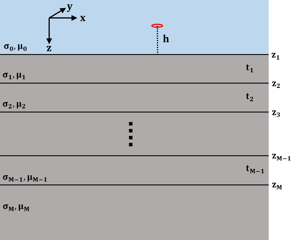
Fig. 2.1 Layered 1D model describing the Earth for each sounding.

EM1DFM and EM1DFMFWD model the Earth’s response for measurements above a stack of uniform, horizontal layers. The coordinate system used for describing the Earth models has z as positive downwards, with the surface of the Earth at z=0. The z-coordinates of the source and receiver locations (which must be above the surface) are therefore negative. Each layer is defined by a thickness, an electrical conductivity, and a magnetic susceptibility (if desired). It is the physical properties of the layers that are obtained during the inversion of all measurements gathered at a single location, with the depths to the layer interfaces remaining fixed. If measurements made at multiple locations are being interpreted, the corresponding one-dimensional models are juxtaposed to create a two-dimensional image of the subsurface.

Because horizontal position is meaningless in a model that varies only vertically, all measurements that are to be inverted for a single one-dimensional model must be grouped together as a “sounding”. A sounding can be considered a distinct collection of FEM measurements (transmitters, receivers and frequencies). Each different sounding is inverted for a separate one-dimensional model. The horizontal location at which a sounding is centered is not used within the program, but is written out to distinguish results for different soundings.

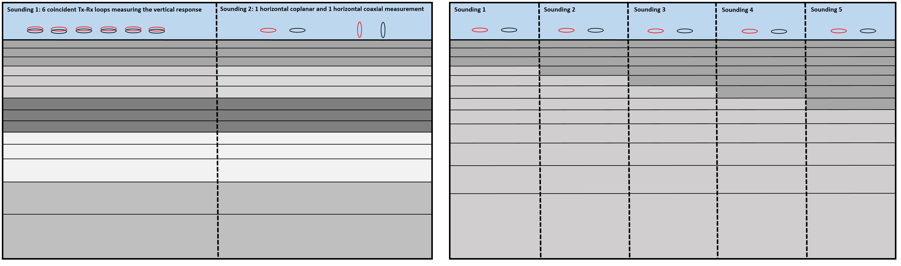
Fig. 2.2 Two distinct groupings of transmitters and receivers (soundings) at the same location (left). Different soundings used to map lateral variation in the Earth (right). Click to enlarge.

The electrical conductivity of Earth materials varies over several orders of magnitude, making it more natural to invert for the logarithms of the layer conductivities rather than the conductivities themselves. This also ensures that conductivities in the constructed model are positive. It is not appropriate, however, to invert for the logarithms of the layer susceptibilities. Near-zero values of susceptibility would become overly important and large values would be overestimated ([]). Therefore susceptibilities are found directly by the inversion, with the option of imposing a positivity constraint.

2.1.3. Details regarding the data

For a magnetic dipole source oriented in the x, y and/or z-direction, EM1DFM and EM1DFMFWD can handle any combination of:

• frequencies for the transmitter current

• separations and heights for the transmitter and receiver(s)

• in phase and quadrature components of the response

• x, y and z-components of the response

Programs EM1DFM and EM1DFMFWD accept observations in four different forms: values of the secondary magnetic field (total minus free-space) normalized by the free-space field and given in parts-per- million, values of the secondary field normalized by the free-space field and given in percent, values of the secondary H-field in A/m, and values of the total H-field in A/m. If the transmitter and receiver have the same orientation, the x-, y- and z-components of the secondary field are normalized by the x-, y- and z-components of the free-space field respectively. If the transmitter and receiver have different orientations, the secondary field is normalized by the magnitude of the free-space field.

2.2. Forward Modeling

Note

This code uses a left-handed coordinate system with X (Easting), Y (Northing) and Z (+ve downwards) with a time-dependency of \(e^{+ i\omega t}\).

The method used to compute the magnetic field values for a particular source-receiver arrangement over a layered Earth model is the matrix propagation approach described in Farquharson ([]). The method uses the z-component of the Schelkunoff F-potential ([]):

(2.1)\[\begin{split}\begin{align} \mathbf{E} &= -\nabla \times \mathbf{F} \\ \mathbf{H} &= -\sigma \mathbf{F} + \dfrac{1}{i \omega \mu} \nabla \big ( \nabla \cdot \mathbf{F} \big ) \end{align}\end{split}\]

where \(\mathbf{E}\), \(\mathbf{H}\), \(\sigma\) and \(\mu\) are the electric field, magnetic field, conductivity and magnetic permeability, respectively, within the uniform region for which this equation is valid. Note that the time-dependence \(e^{i\omega t}\) has been suppressed. The permeability is related to the susceptibility (\(\kappa\)) via the following equation:

(2.2)\[\mu = \mu_0 \big ( 1 + \kappa \big )\]

where \(\mu_0\) is the permeability of free space. In the \(j^{th}\) layer (where \(j>0\)) with conductivity \(\sigma_j\) and permeability \(\mu_j\), the z-component of the Schelkunoff potential satisfies the following equation (assuming the quasi-static approximation):

(2.3)\[\nabla^2 F_j - i\omega \mu_j \sigma_j F = 0\]

Applying the two-dimensional Fourier transform to eq. () gives:

(2.4)\[\frac{d^2 \tilde{F}_j}{dz^2} - u_j^2 \tilde{F}_j = 0\]

where \(u_j^2 = k_x^2 + k_y^2 + i \omega \mu_j \sigma_j\), and \(k_x\) and \(k_y\) are the horizontal wavenumbers. The solution to this equation is:

(2.5)\[\tilde{F}_j (k_x,k_y,z,\omega ) = D_j (k_x, k_y, \omega) \, e^{-u_j (z-z_j)} + U_j (k_x, k_y, \omega) \, e^{u_j (z-z_j)}\]

where \(D_j\) and \(U_j\) are the coefficients of the downward and upward-decaying parts of the solution, respectively. At the interface between layer \(j-1\) and layer \(j\), which is at depth \(z_j\), the conditions on \(\tilde{F}\) are:

(2.6)\[\begin{split}\begin{align} \tilde{F}_{j-1} \Big |_{z=z_j} &= \tilde{F}_j \Big |_{z=z_j}, \\ \dfrac{1}{\mu_{j-1}} \dfrac{d \tilde{F}_{j-1}}{dz} \Bigg |_{z=z_j} &= \dfrac{1}{\mu_{j}} \dfrac{d \tilde{F}_{j}}{dz} \Bigg |_{z=z_j} \end{align}\end{split}\]

Applying these conditions to the solutions for \(j \geq 2\) gives:

(2.7)\[\begin{split}\begin{bmatrix} e^{-u_{j-1} t_{j-1}} & e^{u_{j-1} t_{j-1}} \\ - \frac{u_{j-1}}{\mu_{j-1}} e^{-u_{j-1} t_{j-1}} & \frac{u_{j-1}}{\mu_{j-1}} e^{u_{j-1} t_{j-1}} \end{bmatrix} \begin{bmatrix} D_{j-1} \\ U_{j-1} \end{bmatrix} = \begin{bmatrix} 1 & 1 \\ -\frac{u_j}{\mu_j} & \frac{u_j}{\mu_j} \end{bmatrix} \begin{bmatrix} D_{j} \\ U_{j} \end{bmatrix},\end{split}\]

where \(t_{j-1} = z_j - z_{j-1}\) is the thickness of layer \(j-1\). Through factoring and rearranging, the above equation can be re-expressed as:

(2.8)\[\begin{split}\begin{bmatrix} D_{j-1} \\ U_{j-1} \end{bmatrix} = e^{u_{j-1}t_{j-1}} \mathbf{M_j} \begin{bmatrix} D_{j} \\ U_{j} \end{bmatrix},\end{split}\]

where

(2.9)\[\begin{split}\mathbf{M_j} = \begin{bmatrix} \frac{1}{2} \Big ( 1 + \frac{\mu_{j-1} u_j}{\mu_j u_{j-1}} \Big ) & \frac{1}{2} \Big ( 1 - \frac{\mu_{j-1} u_j}{\mu_j u_{j-1}} \Big ) \\ \frac{1}{2} \Big ( 1 - \frac{\mu_{j-1} u_j}{\mu_j u_{j-1}} \Big ) e^{-2u_{j-1} t_{j-1}} & \frac{1}{2} \Big ( 1 + \frac{\mu_{j-1} u_j}{\mu_j u_{j-1}} \Big ) e^{-2u_{j-1} t_{j-1}} \end{bmatrix} \;\;\;\; \textrm{for} \;\;\;\; j \geq 2\end{split}\]

In layer 0 (the air interface), \(\tilde{F}\) is given by:

(2.10)\[\tilde{F}_0 = D_0 e^{-u_0 z} + U_0 e^{u_0 z},\]

which leads to

(2.11)\[\begin{split}\begin{bmatrix} D_0 \\ U_0 \end{bmatrix} = \mathbf{M_1} \begin{bmatrix} D_1 \\ U_1 \end{bmatrix}\end{split}\]

and

(2.12)\[\begin{split}\mathbf{M_1} = \begin{bmatrix} \frac{1}{2} \Big ( 1 + \frac{\mu_0 u_1}{\mu_1 u_0} \Big ) & \frac{1}{2} \Big ( 1 - \frac{\mu_0 u_1}{\mu_1 u_0} \Big ) \\ \frac{1}{2} \Big ( 1 - \frac{\mu_0 u_1}{\mu_1 u_0} \Big ) & \frac{1}{2} \Big ( 1 + \frac{\mu_0 u_1}{\mu_1 u_0} \Big ) \end{bmatrix}\end{split}\]

Using eqs. () and (), we can relate the coefficients \(U_0\) and \(D_0\) of the solution in the air to the coefficients \(U_M\) and \(D_M\) of the solution in the basement halfspace:

(2.13)\[\begin{split}\begin{bmatrix} D_0 \\ U_0 \end{bmatrix} = \mathbf{M_1} exp \Bigg ( \sum_{j=2}^M u_{j-1} t_{j-1} \Bigg ) \prod_{j=2}^M \mathbf{M_j} \begin{bmatrix} D_M \\ U_M \end{bmatrix}\end{split}\]

There is no upward-decaying part of the solution in the basement halfspace (thus \(U_M = 0\)). In the air, the downward-decaying part is due to the source (thus \(D_0 = D_0^s\)). Eq. () can therefore be rewritten as:

(2.14)\[\begin{split}\begin{bmatrix} D_0^2 \\ U_0 \end{bmatrix} = E \, \mathbf{ P} \begin{bmatrix} D_M \\ 0 \end{bmatrix}\end{split}\]

where the matrix \(\mathbf{P}\) is given by

(2.15)\[\mathbf{P} = \mathbf{M_1} \prod_{j=2}^M \mathbf{M_j}\]

and the factor \(E\) is given by:

(2.16)\[E = exp \Bigg ( \sum_{j=2}^M u_{j-1} t_{j-1} \Bigg )\]

From eq. (), we see that:

(2.17)\[D_M = \frac{1}{E} \frac{1}{P_{11}} D_0^s\]

and

(2.18)\[U_0 = E \, P_{21} \, D_M\]

Substituting the previous two equations gives:

(2.19)\[U_0 = \frac{P_{21}}{P_{11}} D_0^s\]

which does not involve any exponential terms whose arguments have positive real parts, making this formulation inherently stable. The solution for \(\tilde{F}\) in the air halfspace is therefore given by:

(2.20)\[\tilde{F}_0 = D_0^s \Bigg ( e^{-u_0 z} + \frac{P_{21}}{P_{11}} e^{u_0 z} \Bigg )\]

For a unit vertical magnetic dipole source at a height \(h\) (i.e. \(z = -h\) for \(h>0\)) above the surface of the Earth:

(2.21)\[D_0^s = \frac{i\omega \mu_0}{2 u_0}e^{-u_0 h}\]

([], eq. 4.40), and for a unit x-directed magnetic dipole source at \(z=-h\):

(2.22)\[D_0^s = - \frac{i\omega \mu_0}{2} \frac{ik_x}{k_x^2 + k_y^2} e^{-u_0 h}\]

([], eq. 4.106). Once whichever of these terms is appropriate is substituted into eq. (), the solution is completed by converting the required inverse two-dimensional Fourier transform to a Hankel transform, and using eq. () to obtain the three components of the H-field above the Earth model (\(z<0\)). For a z-directed magnetic dipole source at (\(0,0,-h\)) such that \(h>0\):

(2.23)\[\begin{split}\begin{align} H_x(x,y,z,\omega) &= \frac{1}{4\pi} \frac{x}{r} \int_0^\infty \Big ( e^{-\lambda |z+h|} - \frac{P_{21}}{P_{11}} e^{\lambda (z-h)} \Big ) \lambda^2 J_1(\lambda r) d\lambda \\ H_y(x,y,z,\omega) &= \frac{1}{4\pi} \frac{y}{r} \int_0^\infty \Big ( e^{-\lambda |z+h|} - \frac{P_{21}}{P_{11}} e^{\lambda (z-h)} \Big ) \lambda^2 J_1(\lambda r) d\lambda \\ H_z(x,y,z,\omega) &= \frac{1}{4\pi} \int_0^\infty \Big ( e^{-\lambda |z+h|} + \frac{P_{21}}{P_{11}} e^{\lambda (z-h)} \Big ) \lambda^2 J_0(\lambda r) d\lambda \end{align}\end{split}\]

And for a x-directed magnetic dipole source at (\(0,0,-h\)) such that \(h>0\):

(2.24)\[\begin{split}\begin{align} H_x(x,y,z,\omega) =& -\frac{1}{4\pi} \Big ( \frac{1}{r} - \frac{2x^2}{r^3} \Big ) \int_0^\infty \Big ( e^{-\lambda |z+h|} - \frac{P_{21}}{P_{11}} e^{\lambda (z-h)} \Big ) \lambda J_1(\lambda r) d\lambda \\ &-\frac{1}{4\pi} \frac{x^2}{r^2} \int_0^\infty \Big ( e^{-\lambda |z+h|} - \frac{P_{21}}{P_{11}} e^{\lambda (z-h)} \Big ) \lambda^2 J_0(\lambda r) d\lambda \\ H_y(x,y,z,\omega) =& \frac{1}{2\pi} \frac{xy}{r^3} \int_0^\infty \Big ( e^{-\lambda |z+h|} - \frac{P_{21}}{P_{11}} e^{\lambda (z-h)} \Big ) \lambda J_1(\lambda r) d\lambda \\ &-\frac{1}{4\pi} \frac{xy}{r^2} \int_0^\infty \Big ( e^{-\lambda |z+h|} - \frac{P_{21}}{P_{11}} e^{\lambda (z-h)} \Big ) \lambda^2 J_0(\lambda r) d\lambda \\ H_z(x,y,z,\omega) =& \frac{1}{4\pi} \frac{x}{r} \int_0^\infty \Big ( e^{-\lambda |z+h|} + \frac{P_{21}}{P_{11}} e^{\lambda (z-h)} \Big ) \lambda^2 J_1(\lambda r) d\lambda \end{align}\end{split}\]

The Hankel transforms in eqs. () and () are computed using the digital filtering routine of Anderson ([]). The kernels of these equations are pre-computed at a certain number of logarithmically-spaced values of \(\lambda\). Anderson’s routine then extracts the values of the kernels at the values of \(\lambda\) it requires by cubic spline interpolation. The number of values of \(\lambda\) at which the kernels are pre-computed (50 minimum) can be specified in the input file “em1dfm.in”; see “line 11” in the input file description.

There are three places where previously-computed components of eqs. () and () can be re-used. The propagation of the matrices through the layers depends on frequency, and must be re-done for each different value. However, the propagated matrix \(\mathbf{P}\), and hence the ratio \(P_{21}/P_{11}\), does not depend on the relative location and orientation of the transmitter and receiver, and so can be re-used for all transmitters and receivers for the same frequency. Furthermore, if there are multiple transmitter-receiver pairs with the same height (and the same frequency), there is no difference in the kernels of their Hankel transforms, and so the values of the kernels computed for one pair can be re-used for all the others. It is to ensure this grouping of the survey parameters that the observations file is structured the way it is (see the observation file).

The individual propagation matrices \(\mathbf{M_j}\), and each matrix computed in the construction of the propagation matrix \(\mathbf{P}\), are saved in the forward-modelling routine. These are then re-used in the computation of the sensitivities.

2.3. Computing Sensitivities

The inverse problem of determining the conductivity and/or susceptibility of the Earth from electromagnetic measurements is nonlinear. Program EM1DFM uses an iterative procedure to solve this problem. At each iteration the linearized approximation of the full nonlinear problem is solved. This requires the Jacobian matrix for the sensitivities, \(\mathbf{J} = (\mathbf{J^\sigma}, \mathbf{J^\kappa})\) where:

(2.25)\[\begin{split}\begin{align} J_{ij}^\sigma &= \frac{\partial d_i}{\partial log \, \sigma_j} \\ J_{ij}^\kappa &= \frac{\partial d_i}{\partial k_j} \end{align}\end{split}\]

in which \(d_i\) is the \(i^{th}\) observation, and \(\sigma_j\) and \(\kappa_j\) are the conductivity and susceptibility of the \(j^{th}\) layer.

The algorithm for computing the sensitivities is obtained by differentiating the expressions for the H-fields (see () and ()) with respect to the model parameters ([]). For example, the sensitivity with respect to \(m_j\) (either the conductivity or susceptibility of the \(j^{th}\) layer) of the z-component of the H-field for a z-directed magnetic dipole source is given by differentiating the third expression in ():

(2.26)\[\frac{\partial H_z}{\partial m_j} (x,y,z,\omega) = \frac{1}{4\pi} \int_0^\infty \Big ( e^{-\lambda |z+h|} + \frac{\partial}{\partial m_j} \Bigg [ \frac{P_{21}}{P_{11}} \Bigg ] e^{\lambda (z-h)} \Big ) \lambda^2 J_0(\lambda r) d\lambda\]

The derivative of the coefficient is simply:

(2.27)\[\frac{\partial}{\partial m_j} \Bigg [ \frac{P_{21}}{P_{11}} \Bigg ] = \frac{\partial P_{21}}{\partial m_j} \frac{1}{P_{11}} - \frac{\partial P_{11}}{\partial m_j} \frac{P{21}}{P_{11}^2}\]

where \(P_{11}\) and \(P_{21}\) are elements of the propagation matrix \(\mathbf{P}\) given by eq. (). The derivative of \(\mathbf{P}\) with respect to \(m_j\) (for \(1 \leq j \leq M-1\)) is

(2.28)\[\frac{\partial \mathbf{P}}{\partial m_j} = \mathbf{M_1 M_2 ... M_{j-1}} \Bigg ( \frac{\partial \mathbf{M_j}}{\partial m_j} \mathbf{M_{j+1}} + \mathbf{M_j} \frac{\partial \mathbf{M_{j+1}}}{\partial m_j} \Bigg ) \mathbf{M_{j+2} ... M_M}\]

The sensitivities with respect to the conductivity and susceptibility of the basement halfspace are given by

(2.29)\[\frac{\partial \mathbf{P}}{\partial m_M} = \mathbf{M_1 M_2 ... M_{M-1}} \frac{\partial \mathbf{M_M}}{\partial m_M}\]

The derivatives of the individual layer matrices with respect to the conductivities and susceptibilities are straightforward to derive, and are not given here.

Just as for the forward modelling, the Hankel transform in eq. (), and those in the corresponding expressions for the sensitivities of the other observations, are computed using the digital filtering routine of Anderson ([]).

The partial propagation matrices

(2.30)\[\mathbf{P_k} = \mathbf{M_1} \prod_{j=2}^k \mathbf{M_j}, \;\;\; k=2,...,M\]

are computed during the forward modelling, and saved for re-use during the sensitivity computations. This sensitivity-equation approach therefore has the efficiency of an adjoint-equation approach.

2.4. Inversion Methodologies

In program EM1DFM, there are four different inversion algorithms. They all have the same general formulation, but differ in their treatment of the trade-off parameter (see fixed trade-off, discrepency principle, GCV and L-curve criterion). In addition, there are four possibilities for the Earth model constructed by the inversion:

1. conductivity only

2. susceptibility only (with positivity enforced)

3. conductivity and susceptibility (with positivity of the susceptibilities enforced)

4. conductivity and susceptibility (without the positivity constraint)

2.4.1. General formulation

The aim of each inversion algorithm is to construct the simplest model that adequately reproduces the observations. This is achieved by posing the inverse problem as an optimization problem in which we recover the model that minimizes the objective function:

(2.31)\[\Phi = \phi_d + \beta \phi_m - \gamma \phi_{LB}\]

The three components of this objective function are as follows. \(\phi_d\) is the data misfit:

(2.32)\[\phi_d = \| \mathbf{W_d} (\mathbf{d - d^{obs}} ) \|^2\]

where \(\| \, \cdot \, \|\) represents the \(l_2\)-norm, \(d^{obs}\) is the vector containing the \(N\) observations, and \(d\) is the forward-modelled data. It is assumed that the noise in the observations is Gaussian and uncorrelated, and that the estimated standard deviation of the noise in the \(i^{th}\) observation is of the form \(s_0 \hat{s}_i\), where \(\hat{s}_i\) indicates the amount of noise in the \(i^{th}\) observation relative to that in the others, and is a scale factor that specifies the total amount of noise in the set of observations. The matrix \(\mathbf{W_d}\) is therefore given by:

(2.33)\[\mathbf{W_d} = \textrm{diag} \big \{ 1/(s_0 \hat{s}_1), ..., 1/(s_0 \hat{s}_N) \}\]

The model-structure component of the objective function is \(\phi_m\). In its most general form it contains four terms:

(2.34)\[\begin{split}\begin{split} \phi_m =& \; \alpha_s^\sigma \big \| \mathbf{W_s^\sigma} \big ( \mathbf{m^\sigma - m_s^{\sigma , ref}} \big ) \big \|^2\\ &+ \alpha_z^\sigma \big \| \mathbf{W_z^\sigma} \big ( \mathbf{m^\sigma - m_z^{\sigma , ref}} \big ) \big \|^2\\ &+ \alpha_s^\kappa \big \| \mathbf{W_s^\kappa} \big ( \mathbf{m^\kappa - m_s^{\kappa , ref}} \big ) \big \|^2\\ &+ \alpha_z^\kappa \big \| \mathbf{W_z^\kappa} \big ( \mathbf{m^\kappa - m_z^{\kappa , ref}} \big ) \big \|^2 \end{split}\end{split}\]

where \(\mathbf{m^\sigma}\) is the vector containing the logarithms of the layer conductivities, and \(\mathbf{m^\kappa}\) is the vector containing the layer susceptibilities. The matrices \(\mathbf{W_s^\sigma}\) and \(\mathbf{W_s^\kappa}\) are:

(2.35)\[\mathbf{W_s^\sigma} = \mathbf{W_s^\kappa} = \textrm{diag} \big \{ \sqrt{t_1}, ..., \sqrt{t_{m-1}}, \sqrt{t_{M-1}} \big \}\]

where \(t_j\) is the thickness of the \(j^{th}\) layer. And the matricies \(\mathbf{W_z^\sigma}\) and \(\mathbf{W_z^\kappa}\) are:

(2.36)\[\begin{split}\mathbf{W_z^\sigma} = \mathbf{W_z^\kappa} = \begin{bmatrix} -\sqrt{\frac{2}{t_1 + t_2}} & \sqrt{\frac{2}{t_1 + t_2}} & & & & \\ & -\sqrt{\frac{2}{t_2 + t_3}} & \sqrt{\frac{2}{t_2 + t_3}} & & & \\ & & \ddots & & & \\ & & & -\sqrt{\frac{2}{t_{M-2} + t_{M-1}}} & \sqrt{\frac{2}{t_{M-2} + t_{M-1}}} & \\ & & & & -\sqrt{\frac{2}{t_{M-1}}} & \sqrt{\frac{2}{t_{M-1}}} \\ & & & & & 0 \end{bmatrix}\end{split}\]

The rows of any of these four weighting matrices can be scaled if desired (see file for additional model-norm weights). The vectors \(\mathbf{m_s^{\sigma , ref}}\), \(\mathbf{m_z^{\sigma , ref}}\), \(\mathbf{m_s^{\kappa , ref}}\) and \(\mathbf{m_z^{\kappa , ref}}\) contain the layer conductivities/susceptibilities for the four possible reference models. The four terms in \(\phi_m\) therefore correspond to the “smallest” and “flattest” terms for the conductivity and susceptibility parts of the model. The relative importance of the four terms is governed by the coefficients \(\mathbf{\alpha_s^{\sigma}}\), \(\mathbf{\alpha_z^{\sigma}}\), \(\mathbf{\alpha_s^{\kappa}}\) and \(\mathbf{\alpha_z^{\kappa}}\) , which are discussed in the general formulation of the inversion problem. \(\beta\) is the trade-off parameter that balances the opposing effects of minimizing the misfit and minimizing the amount of structure in the model. It is the different ways in which \(\beta\) is determined that distinguish the four inversion algorithms in program EM1DFM from one another. They are described in the next sections.

Finally, the third component of the objective function is a logarithmic barrier term:

(2.37)\[\phi_{LB} = \sum_{j-1}^M \textrm{log} \, (c\kappa_j)\]

where \(c\) is a constant, usually equal to 1. This term is how the positivity constraint on the layer susceptibilities is enforced. It, and its coefficient \(\gamma\), are described here.

As mentioned in the computing sensitivities section, the inverse problem considered here is nonlinear. It is solved using an iterative procedure. At the \(n^{th}\) iteration, the actual objective function being minimized is:

(2.38)\[\Phi^n = \phi_d^n + \beta^n \phi_m^n - \gamma^n \phi^n_{LB}\]

In the data misfit \(\phi_d^n\), the forward-modelled data \(d_n\) are the data for the model that is sought at the current iteration. These data are approximated by:

(2.39)\[\mathbf{d^n} = \mathbf{d}^{n-1} + \mathbf{J}^{\sigma, n-1} \delta \mathbf{m}^\sigma + \mathbf{J}^{\kappa, n-1} \delta \mathbf{m}^\kappa\]

where \(\delta \mathbf{m}^\sigma = \mathbf{m}^{\sigma , n} - \mathbf{m}^{\sigma , n-1}\;\) & \(\;\delta \mathbf{m}^\kappa = \mathbf{m}^{\kappa , n} - \mathbf{m}^{\kappa , n-1}\), and \(\mathbf{J}^{\sigma , n-1}\) & \(\mathbf{J}^{\kappa , n-1}\) are the two halves of the Jacobian matrix given by () and evaluated for the model from the previous iteration. At the \(n^{th}\) iteration, the problem to be solved is that of finding the change, (\(\delta \mathbf{m}^\sigma , \delta \mathbf{m}^\kappa\)) to the model which minimizes the objective function \(\Phi^n\). Differentiating eq. () with respect to the components of \(\delta \mathbf{m}^\sigma\) & \(\delta \mathbf{m}^\kappa\), and equating the resulting expressions to zero, gives the system of equations to be solved. The derivatives of \(\phi^n_d\) (incorporating the approximation of eq. ()) and are straightforward to calculate. However, a further approximation must be made to linearize the derivatives of the logarithmic barrier term:

(2.40)\[\begin{split}\begin{split} \frac{\partial \phi^n_{LB}}{\partial \delta m_k^\kappa} &= \frac{\partial}{\partial \delta \kappa_k} \sum_{j=1}^M \textrm{log} \big ( \kappa_j^{n-1} + \delta \kappa_j \big ) \\ &= \frac{1}{\kappa_k^{n-1} + \delta \kappa_j} \\ & \approx \frac{1}{\kappa_k^{n-1}} \Bigg ( 1 - \frac{\delta \kappa_k}{\kappa_k^{n-1}} \Bigg ) \end{split}\end{split}\]

The linear system of equations to be solved for (\(\delta \mathbf{m}^\sigma , \delta \mathbf{m}^\kappa\)) is therefore:

(2.41)\[\begin{split}\begin{split} & \bigg [ \mathbf{J}^{n-1 \, T} \mathbf{W_d}^T \mathbf{W_d} \mathbf{J}^{n-1} + \beta^n \sum_{i=1}^2 \mathbf{W_i}^T \mathbf{W_i} + \frac{\gamma^n}{2} \mathbf{\hat{X}}^{n-1 \, T} \mathbf{\hat{X}}^{n-1} \bigg ] \delta \mathbf{m} = \\ & \mathbf{J}^{n-1 \, T} \mathbf{W_d}^{n-1} \mathbf{W_d} \big ( \mathbf{d^{obs}} - \mathbf{d}^{n-1} \big ) + \beta^n \sum_{i=1}^2 \mathbf{W_i}^T \mathbf{W_i} \big ( \mathbf{m_i^{ref} - \mathbf{m}^{n-1}} \big ) + \frac{\gamma^n}{2} \mathbf{\hat{X}}^{n-1 \, T} \mathbf{\hat{X}}^{n-1} \mathbf{m}^{n-1} \end{split}\end{split}\]

where \(T\) denotes the transpose and:

(2.42)\[\begin{split}\begin{split} \mathbf{J}^{n-1} &= \big ( \mathbf{J}^{\sigma , n-1} \mathbf{J}^{\kappa , n-1} \big ) \\ \mathbf{W_1} &= \begin{bmatrix} \sqrt{\alpha_s^\sigma} \mathbf{W}_s^\sigma & 0 \\ 0 & \sqrt{\alpha_s^\kappa} \mathbf{W}_s^\kappa \end{bmatrix} \\ \mathbf{W_2} &= \begin{bmatrix} \sqrt{\alpha_z^\sigma} \mathbf{W}_z^\sigma & 0 \\ 0 & \sqrt{\alpha_z^\kappa} \mathbf{W}_z^\kappa \end{bmatrix} \\ \mathbf{m_1^{ref}} &= \big ( \mathbf{m}_s^{\sigma , ref \, T} \mathbf{m}_s^{\kappa , ref \, T} \big )^T \\ \mathbf{m_2^{ref}} &= \big ( \mathbf{m}_z^{\sigma , ref \, T} \mathbf{m}_z^{\kappa , ref \, T} \big )^T \\ \mathbf{\hat{X}}^{n-1} &= \big ( 0 \, (\mathbf{X}^{n-1})^{-1} \big ) \end{split}\end{split}\]

where \(\mathbf{\hat{X}}^{n-1} = \textrm{diag} \{ m_1^{\kappa, n-1}, ... , m_M^{\kappa, n-1} \}\). The solution to eq. () is equivalent to the least-squares solution of:

(2.43)\[\begin{split}\begin{bmatrix} \mathbf{W_d J}^{n-1} \\ \sqrt{\beta^n} \mathbf{W_1} \\ \sqrt{\beta^n} \mathbf{W_2} \\ \sqrt{\gamma^n/2} \, \mathbf{\hat{X}}^{n-1} \end{bmatrix} \delta \mathbf{m} = \begin{bmatrix} \mathbf{W_d } ( \mathbf{d^{obs} - d}^{n-1} ) \\ \sqrt{\beta^n} \mathbf{W_1} ( \mathbf{m_1^{ref} - m}^{n-1} ) \\ \sqrt{\beta^n} \mathbf{W_2}( \mathbf{m^{ref} - m}^{n-1} ) \\ \sqrt{\gamma^n/2} \, \mathbf{\hat{X}}^{n-1} \mathbf{m}^{n-1} \end{bmatrix}\end{split}\]

Once the step \(\delta \mathbf{m}\) has been determined by the solution of eq. () or eq. (), the new model is given by:

(2.44)\[\mathbf{m}^n = \mathbf{m}^{n-1} + \nu \delta \mathbf{m}\]

There are two conditions on the step length \(\nu\). First, if positivity of the layer susceptibilities is being enforced:

(2.45)\[\nu \delta \kappa_j > -\kappa_j^{n-1}\]

must hold for all \(j=1,...,M\). Secondly, the objective function must be decreased by the addition of the step to the model:

(2.46)\[\phi_d^n + \beta^n \phi_m^n - \gamma^n \phi_{LB}^n < \phi_d^{n-1} + \beta^n \phi_m^{n-1} - \gamma^n \phi_{LB}^{n-1}\]

where \(\phi_d^n\) is now the misfit computed using the full forward modelling for the new model \(\mathbf{m}^n\). To determine \(\mathbf{m}^n\), a step length (\(\nu\)) of either 1 or the maximum value for which eq. () is true (whichever is greater) is tried. If eq. () is true for the step length, it is accepted. If eq. () is not true, \(\nu\) is decreased by factors of 2 until it is true.

2.4.2. Algorithm 1: fixed trade-off parameter

The trade-off parameter, \(\beta\), remains fixed at its user-supplied value throughout the inversion. The least- squares solution of eq. () is used. This is computed using the subroutine “LSQR” of Paige & Saunders ([]). If the desired value of \(\beta\) is known, this is the fastest of the four inversion algorithms as it does not involve a line search over trial values of \(\beta\) at each iteration. If the appropriate value of \(\beta\) is not known, it can be found using this algorithm by trail-and-error. This may or may not be time-consuming.

2.4.3. Algorithm 2: discrepancy principle

If a complete description of the noise in a set of observations is available - that is, both \(s_0\) and \(\hat{s}_i \: (i=1,...,N)\) are known - the expectation of the misfit, \(E (\phi_d)\), is equal to the number of observations \(N\). Algorithm 2 therefore attempts to choose the trade-off parameter so that the misfit for the final model is equal to a target value of \(chifac \times N\). If the noise in the observations is well known, \(chifac\) should equal 1. However, \(chifac\) can be adjusted by the user to give a target misfit appropriate for a particular data-set. If a misfit as small as the target value cannot be achieved, the algorithm searches for the smallest possible misfit.

Experience has shown that choosing the trade-off parameter at early iterations in this way can lead to excessive structure in the model, and that removing this structure once the target (or minimum) misfit has been attained can require a significant number of additional iterations. A restriction is therefore placed on the greatest-allowed decrease in the misfit at any iteration, thus allowing structure to be slowly but steadily introduced into the model. In program EM1DFM, the target misfit at the \(n^{th}\) iteration is given by:

(2.47)\[\phi_d^{n, tar} = \textrm{max} \big ( mfac \times \phi_d^{n-1}, chifac \times N \big )\]

where the user-supplied factor \(mfac\) is such that \(0.1 \leq mfac \leq 0.5\).

The step \(\delta \mathbf{m}\) is found from the solution of eq. () using subroutine LSQR of Paige & Saunders ([]). The line search at each iteration moves along the \(\phi_d\) versus log \(\! \beta\) curve until either the target misfit, \(\phi_d^{n, tar}\), is bracketed, in which case a bisection search is used to converge to the target, or the minimum misfit (\(> \phi_d^{n-1}\)) is bracketed, in which case a golden section search (for example, Press et al., 1986) is used to converge to the minimum. The starting value of \(\beta\) for each line search is \(\beta^{n-1}\). For the first iteration, the \(\beta \, (=\beta_0)\) for the line search is given by \(N/\phi_m (\mathbf{m}^\dagger)\), where \(\mathbf{m}^\dagger\) contains typical values of conductivity and/or susceptibility. Specifically, \(\mathbf{m}^\dagger\) is a model whose top \(M/5\) layers have a conductivity of 0.02 S/m and susceptibility of 0.02 SI units, and whose remaining layers have a conductivity of 0.01 S/m and susceptibility of 0 SI units. Also, the reference models used in the computation of \(\phi_m (\mathbf{m}^\dagger )\) are homogeneous halfspaces of 0.01 S/m and 0 SI units. The line search is efficient, but does involve the full forward modelling to compute the misfit for each trial value of \(\beta\).

2.4.4. Algorithm 3: GCV criterion

If only the relative amount of noise in the observations is known - that is, \(\hat{s}_i (i=1,...,N)\) is known but not \(s_0\) - the appropriate target value for the misfit cannot be determined, and hence Algorithm 2 is not the most suitable. The generalized cross-validation (GCV) method provides a means of estimating, during the course of an inversion, a value of the trade-off parameter that results in an appropriate fit to the observations, and in so doing, effectively estimating the level of noise, \(s_0\), in the observations (see, for example, []; []).

The GCV method is based on the following argument ([]; []; []). Consider inverting all but the first observation using a trial value of \(\beta\), and then computing the individual misfit between the first observation and the first forward-modelled datum for the model produced by the inversion. This can be repeated leaving out all the other observations in turn, inverting the retained observations using the same value of \(\beta\), and computing the misfit between the observation left out and the corresponding forward-modelled datum. The best value of \(\beta\) can then be defined as the one which gives the smallest sum of all the individual misfits. For a linear problem, this corresponds to minimizing the GCV function. For a nonlinear problem, the GCV method can be applied to the linearized problem being solved at each iteration ([]; []; []; []). From eq. (), the GCV function for the \(n^{th}\) iteration is given by:

(2.48)\[GCV (\beta ) = \dfrac{\big \| \mathbf{W_d \hat{d} - W_d J}^{n-1} \mathbf{M}^{-1} \big ( \mathbf{J}^{n-1 \, T} \mathbf{W_d}T \mathbf{W_d \hat{d} + r} \big ) \big \|^2 }{\big [ \textrm{trace} \big ( \mathbf{I - W_d J}^{n-1} \mathbf{M}^{-1} \mathbf{J}^{n-1 \, T} \mathbf{W_d}^T \big ) \big ]^2}\]

where

(2.49)\[\begin{split}\begin{split} \mathbf{M} (\beta) &= \bigg [ \mathbf{J}^{n-1 \, T} \mathbf{W_d}^T \mathbf{W_d} \mathbf{J}^{n-1} + \beta^n \sum_{i=1}^2 \mathbf{W_i}^T \mathbf{W_i} + \frac{\gamma^n}{2} \mathbf{\hat{X}}^{n-1 \, T} \mathbf{\hat{X}}^{n-1} \bigg ] \\ \mathbf{r} &= \beta^n \sum_{i=1}^2 \mathbf{W_i}^T \mathbf{W_i} \big ( \mathbf{m_i^{ref} - \mathbf{m}^{n-1}} \big ) + \frac{\gamma^n}{2} \mathbf{\hat{X}}^{n-1 \, T} \mathbf{\hat{X}}^{n-1} \mathbf{m}^{n-1} \end{split}\end{split}\]

and \(\mathbf{\hat{d} - d^{obs} - d}^{n-1}\). If \(\beta^*\) is the value of the trade-off parameter that minimizes eq. () at the \(n^{th}\) iteration, the actual value of \(\beta\) used to compute the new model is given by:

(2.50)\[\beta_n = \textrm{max} (\beta^*, bfac \times \beta^{n-1} )\]

where the user-supplied factor \(bfac\) is such that \(0.01<bfac<0.5\). As for Algorithm 2, this limit on the allowed decrease in the trade-off parameter prevents unnecessary structure being introduced into the model at early iterations. The inverse of the matrix \(\mathbf{M}\) required in eq. (), and the solution to eq. () given this inverse, is computed using the Cholesky factorization routines from LAPACK ([]). The line search at each iteration moves along the curve of the GCV function versus the logarithm of the trade-off parameter until the minimum is bracketed (or \(bfac \times \beta^{n-1}\) reached), and then a golden section search (e.g., Press et al., 1986) is used to converge to the minimum. The starting value of \(\beta\) in the line search is \(\beta^{n-1}\) ( \(\beta^0\) is estimated in the same way as for Algorithm 2). This is an efficient search, even with the inversion of the matrix \(\mathbf{M}\).

2.4.5. Algorithm 4: L-curve criterion

As for the GCV-based method, the L-curve method provides a means of estimating an appropriate value of the trade-off parameter if only \(\hat{s}_i, \, i=1,...,N\) are known and not \(s_0\). For a linear inverse problem, if the data misfit \(\phi_d\) is plotted against the model norm \(\phi_m\) for all reasonable values of the trade-off parameter \(\beta\), the resulting curve tends to have a characteristic “L”-shape, especially when plotted on logarithmic axes (see, for example, []). The corner of this L-curve corresponds to roughly equal emphasis on the misfit and model norm during the inversion. Moving along the L-curve away from the corner is associated with a progressively smaller decrease in the misfit for large increases in the model norm, or a progressively smaller decrease in the model norm for large increases in the misfit. The value of \(\beta\) at the point of maximum curvature on the L-curve is therefore the most appropriate, according to this criterion.

For a nonlinear problem, the L-curve criterion can be applied to the linearized inverse problem at each iteration (Li & Oldenburg, 1999; Farquharson & Oldenburg, 2000). In this situation, the L-curve is defined using the linearized misfit, which uses the approximation given in eq. () for the forward-modelled data. The curvature of the L-curve is computed using the formula (Hansen, 1998):

(2.51)\[C(\beta) = \frac{\zeta^\prime \eta^{\prime \prime } - \zeta^{\prime\prime} \eta^\prime}{\big ( (\zeta^\prime)^2 + (\eta^\prime)^2 \big )^{3/2}}\]

where \(\zeta = \textrm{log} \, \phi_d^{lin}\) and \(\eta = \textrm{log}\, \phi_m\). The prime denotes differentiation with respect to log \(\beta\). As for both Algorithms 2 & 3, a restriction is imposed on how quickly the trade-off parameter can be decreased from one iteration to the next. The actual value of \(\beta\) chosen for use at the \(n^{th}\) th iteration is given by eq. (), where \(\beta^*\) now corresponds to the value of \(\beta\) at the point of maximum curvature on the L-curve.

Experience has shown that the L-curve for the inverse problem considered here does not always have a sharp, distinct corner. The associated slow variation of the curvature with \(\beta\) can make the numerical differentiation required to evaluate eq. () prone to numerical noise. The line search along the L-curve used in program EM1DFM to find the point of maximum curvature is therefore designed to be robust (rather than efficient). The L-curve is sampled at equally-spaced values of \(\textrm{log} \, \beta\), and long differences are used in the evaluation of eq. () to introduce some smoothing. A parabola is fit through the point from the equally-spaced sampling with the maximum value of curvature and its two nearest neighbours. The value of \(\beta\) at the maximum of this parabola is taken as \(\beta^*\). In addition, it is sometimes found that, for the range of values of \(\beta\) that are tried, the maximum value of the curvature of the L-curve on logarithmic axes is negative. In this case, the curvature of the L-curve on linear axes is investigated to find a maximum. As for Algorithms 1 & 2, the least-squares solution to eq. () is used, and is computed using subroutine LSQR of Paige & Saunders ([]).

2.4.6. Relative weighting within the model norm

The four coefficients in the model norm (see eq. ()) are ultimately the responsibility of the user. Larger values of \(\alpha_s^\sigma\) relative to \(\alpha_z^\sigma\) result in constructed conductivity models that are closer to the supplied reference model. Smaller values of \(\alpha_s^\sigma\) and \(\alpha_z^\sigma\) result in flatter conductivity models. Likewise for the coefficients related to susceptibilities.

If both conductivity and susceptibility are active in the inversion, the relative size of \(\alpha_s^\sigma\) & \(\alpha_z^\sigma\) to \(\alpha_s^\kappa\) & \(\alpha_z^\kappa\) is also required. Program EM1DFM includes a simple means of calculating a default value for this relative balance. Using the layer thicknesses, weighting matrices \(\mathbf{W_s^\sigma}\), \(\mathbf{W_z^\sigma}\), \(\mathbf{W_s^\kappa}\) & \(\mathbf{W_z^\kappa}\), and user-supplied weighting of the smallest and flattest parts of the conductivity and susceptibility components of the model norm (see acs, acz, ass & asz in the input file description, line 5), the following two quantities are computed for a test model \(\mathbf{m}^*\):

(2.52)\[\begin{split}\begin{split} \phi_m^\sigma &= acs \big \| \mathbf{W_s^\sigma} \big ( \mathbf{m}^* - \mathbf{m}_s^{\sigma, ref} \big ) \big \|^2 + acz \big \| \mathbf{W_z^\sigma} \big ( \mathbf{m}^* - \mathbf{m}_z^{\sigma, ref} \big ) \big \|^2 \\ \phi_m^\kappa &= ass \big \| \mathbf{W_s^\kappa} \big ( \mathbf{m}^* - \mathbf{m}_s^{\kappa, ref} \big ) \big \|^2 + asz \big \| \mathbf{W_z^\kappa} \big ( \mathbf{m}^* - \mathbf{m}_z^{\kappa, ref} \big ) \big \|^2 \end{split}\end{split}\]

The conductivity and susceptibility of the top \(N/5\) layers in the test model are 0.02 S/m and 0.02 SI units respectively, and the conductivity and susceptibility of the remaining layers are 0.01 S/m and 0 SI units. The coefficients of the model norm used in the inversion are then \(\alpha_s^\sigma = acs\), \(\alpha_z^\sigma = acz\), \(\alpha_s^\kappa = A^s \times ass\) & \(\alpha_z^\kappa = A^d \times asz\) where \(A^s \phi_m^\sigma / \phi_m^\kappa\). It has been found that a balance between the conductivity and susceptibility portions of the model norm computed in this way is adequate as an initial guess. However, the balance usually requires modification by the user to obtain the best susceptibility model. (The conductivity model tends to be insensitive to this balance.) If anything, the default balance will suppress the constructed susceptibility model.

2.4.7. Positive susceptibility

ProgramEM1DFM can perform an unconstrained inversion for susceptibilities (along with the conductivities) as well as invert for values of susceptibility that are constrained to be positive. Following Li & Oldenburg ([]), the positivity constraint is implemented by incorporating a logarithmic barrier term in the objective function (see eqs. () & ()). For the initial iteration, the coefficient of the logarithmic barrier term is chosen so that this term is of equal important to the rest of the objective function:

(2.53)\[\gamma^0 = \frac{\phi_d^0 + \beta^0 \phi_m^0}{- \phi^0_{LB}}\]

At subsequent iterations, the coefficient is reduced according to the formula:

\[\gamma^n = \big ( 1 - \textrm{min}(\nu^{n-1}, 0.925) \big ) \gamma^{n-1}\]

where \(\nu^{n-1}\) is the step length used at the previous iteration. As mentioned at the end of the general formulation, when positivity is being enforced, the step length at any particular iteration must satisfy eq. ().

2.4.8. Convergence criteria

To determine when an inversion algorithm has converged, the following criteria are used ([]):

(2.54)\[\begin{split}\begin{split} \Phi^{n-1} - \Phi^n &< \tau (1 + \Phi^n )\\ \| \mathbf{m}^{n-1} - \mathbf{m} \| &< \sqrt{\tau} (1 + \| \mathbf{m}^n \| ) \end{split}\end{split}\]

where \(\tau\) is a user-specified parameter. The algorithm is considered to have converged when both of the above equations are satisfied. The default value of \(\tau\) is 0.01.

In case the algorithm happens directly upon the minimum, an additional condition is tested:

(2.55)\[\| \mathbf{g}^n \| \leq \epsilon\]

where \(\epsilon\) is a small number close to zero, and where the gradient, \(\mathbf{g}^n\), at the \(n^{th}\) iteration is given by:

(2.56)\[\mathbf{g}^n = -2 \mathbf{J}^{n \, T} \mathbf{W_d}^T \mathbf{W_d} ( \mathbf{d^{obs}} - \mathbf{d}^n ) - 2 \beta^n \sum_{i=1}^2 \mathbf{W_i}^T \mathbf{W_i} \big ( \mathbf{m_i^{ref} - \mathbf{m}^{n-1}} \big ) - \gamma^n \mathbf{\hat{X}}^{n2T} \mathbf{m}^{n}\]